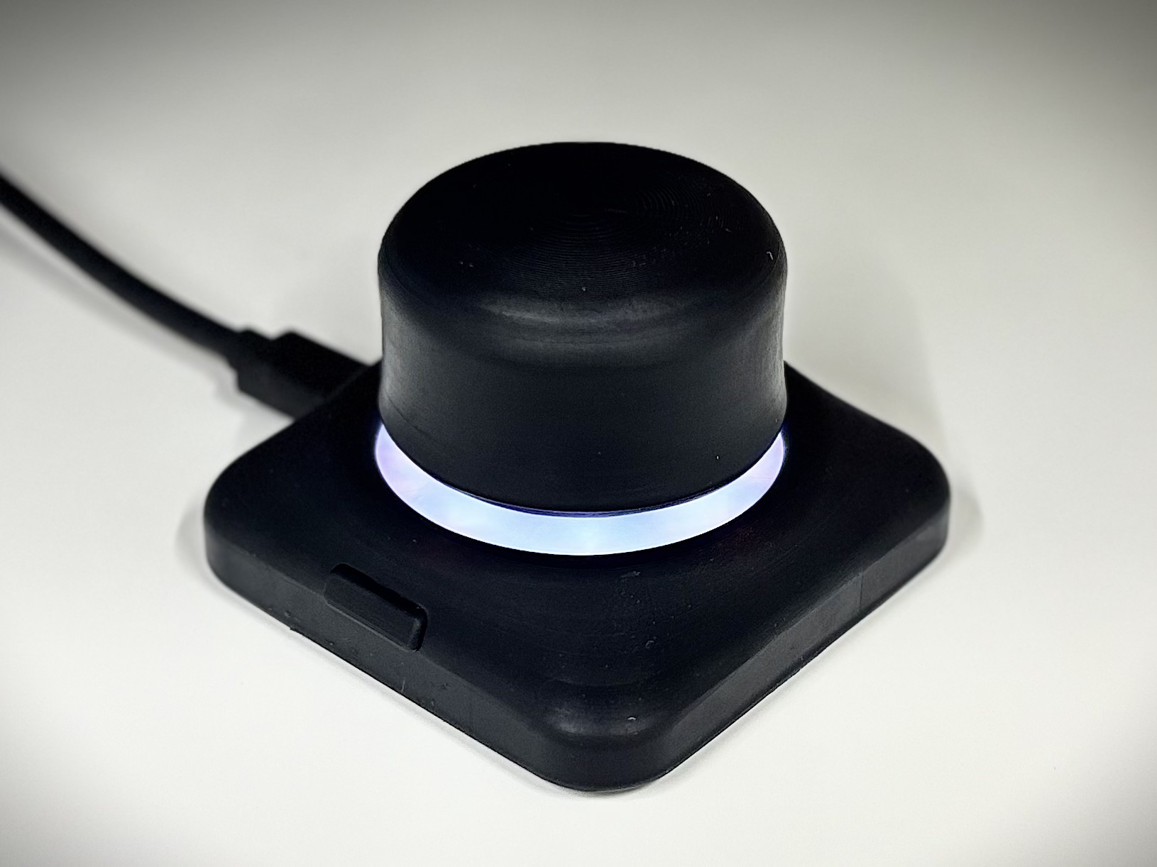
I wanted some kind of mouse for CAD that feels more natural but a real space mouse is $200, so I decided to make my own after PCBWay sponsored this project. The Cosmic Mouse is a 6DOF mouse with a knob which floats in space, it's inspired by the SpaceMouse Compact by 3DConexion. In this post I will walk through the design process of the hardware (PCBs, enclosure), physics model, and firmware which you can find in the Github Repo.
TLDR: I am using 3x 3D Hall effect sensors to pick up the magnets embedded in the knob. The knob floats in space with a custom single-piece isotropic spring. Firmware compensates for magnetic cross-talk by using a physics-based magnetic dipole model and the Levenberg-Marquardt algorithm to iteratively solve for the knob's pose by minimizing the difference between measured and predicted magnetic fields (see the model section). The enclosure knob, and diffuser are resin printed vis MSLA for smoothness. The knob shaft is printed in PETG and sping in TPU. I also used a steel base weight and non-slip silicone pad to keep it planted during movements.
The Cosmic Mouse is very likely capable of emulating a real Space Mouse... On an unrelated note, you should see firmware/src/config.h for some random funny strings.
Hardware (PCBs)
I designed the PCB first with the idea that the layout/spacing of the Hall effect sensors and LEDs would dictate the size of the CAD model. I also did some studies on knob shaft sizing and math for how far the hall effect sensors could be from the magnets.
Microcontroller: I chose an RP2350 based Seeed Studio XIAO over the RP2040 since the RP2350 has hardware support for floating point calculations which is needed for the physics model.
Sensors: For the Hall effect sensors I chose the TMAG5273A1QDBVR, TMAG5273B1QDBVR, and TMAG5273C1QDBVR 3D Hall effect sensors, these are all the same TMAG5273 series but us the A1, B1, and C1 sub models which have different I2C addresses so they can all be put on the same com line without conflict (and no need for delayed power switching address assignment). The A1/B1/C1 models (40/80mT) have lower, but less noisy measurements over the A2/B2/C2 units (133/266mT). Since the knob is only 6DOF I only need 2 sensors, but for greater accuracy I used 3 sensors to to filter noise and absorb hardware imperfections. I considered using 3D TMR sensors, but there were no package sizes which were hand-soldering friendly.
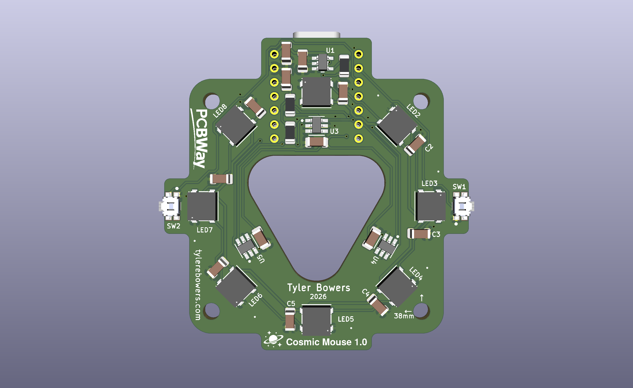
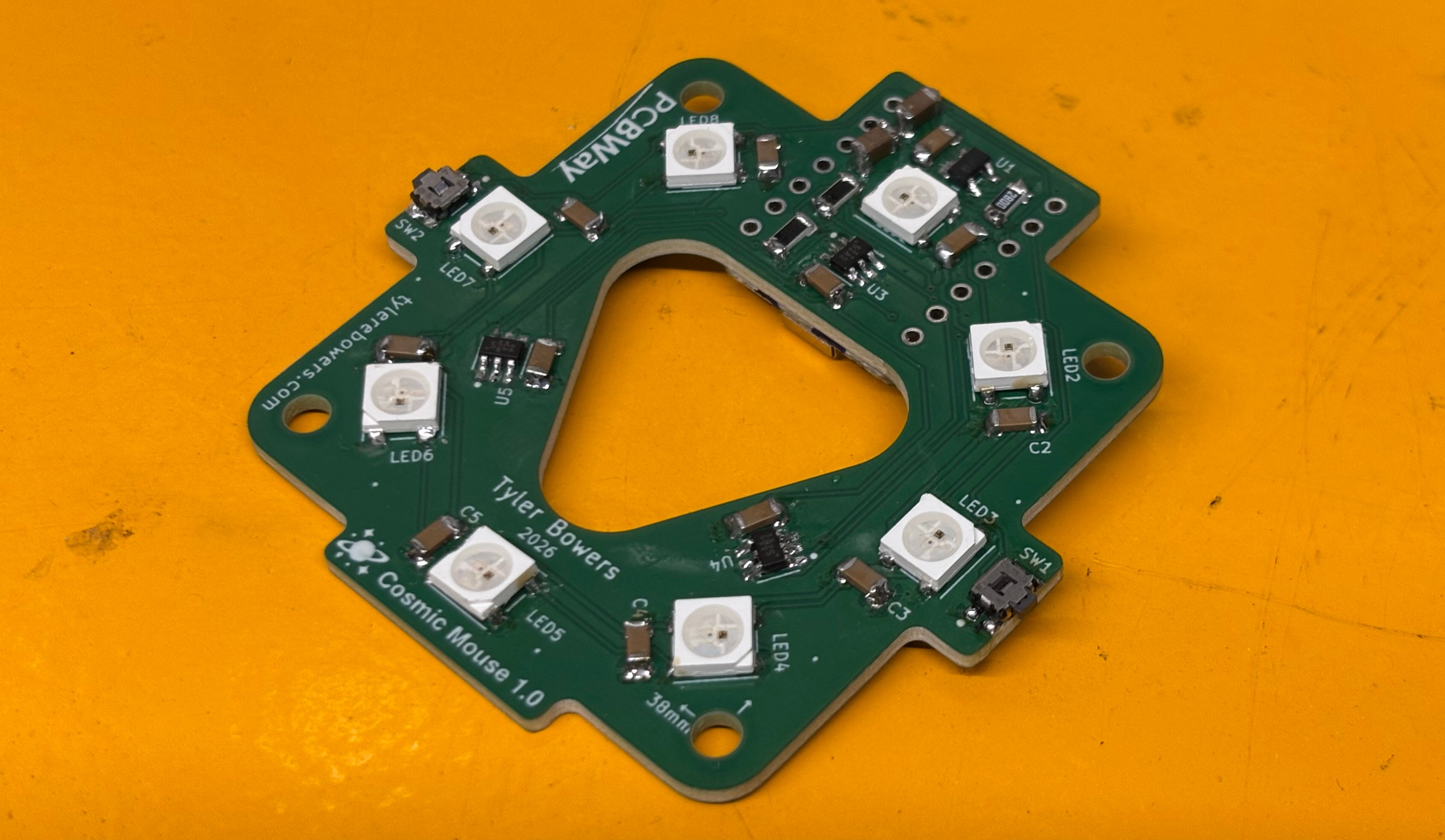
LEDs: The LED ring uses a logic level shifter inline with serial-based coms. The idea behind the ring was that the knob would have a "hovering" if it was over a white ring, the LED ring also communicates to the user when it is calibrating.
The sensors are arranged in a 14.5mm radius about the center z axis with 120 degree spacing. The 8x LED ring is outside of the sensor ring, in hindsight I should have used horizontal LEDs instead of vertical LEDs so they would be more diffuse, though the diffuser does do a good job of de-peaking the LEDs.
Enclosure
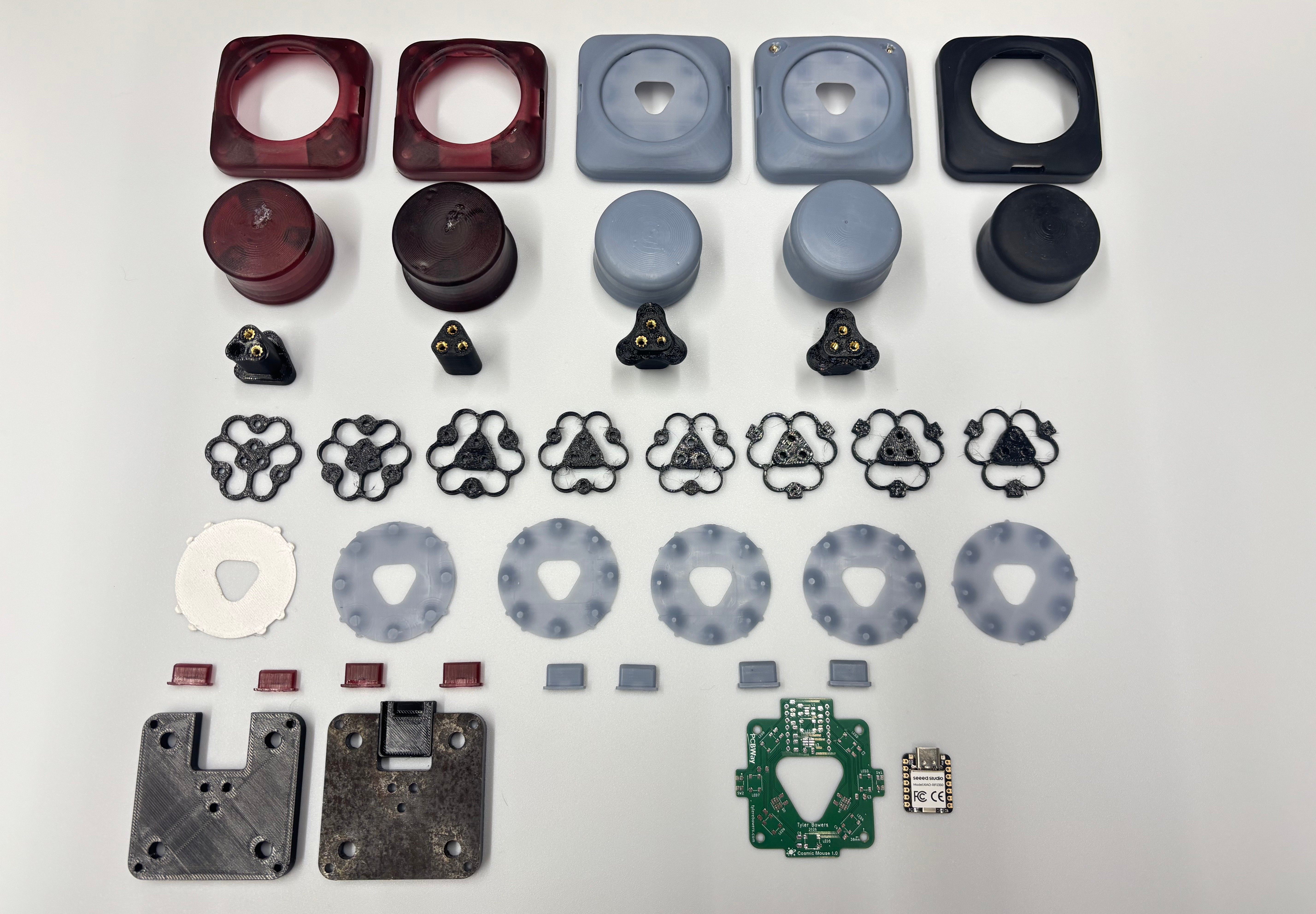
The idea behind the model is simple: a knob floats over a heavy base. I started from the PCB to design the base. The PCB is mounted to the base with glued in heat-set inserts (heat-set inserts do not work with resin prints so they must be glued; in my experience the resin snaps before the JBweld glue give up). I considered snaps but wanted something that was easy to disassemble. The weight is also held in with glued heat-set inserts, but these are separate inserts, since the mouse sits on the weight any impacts should be absorbed by the base to isolate the PCB. Under the weight is a silicone pad to keep the mouse planted during movement.
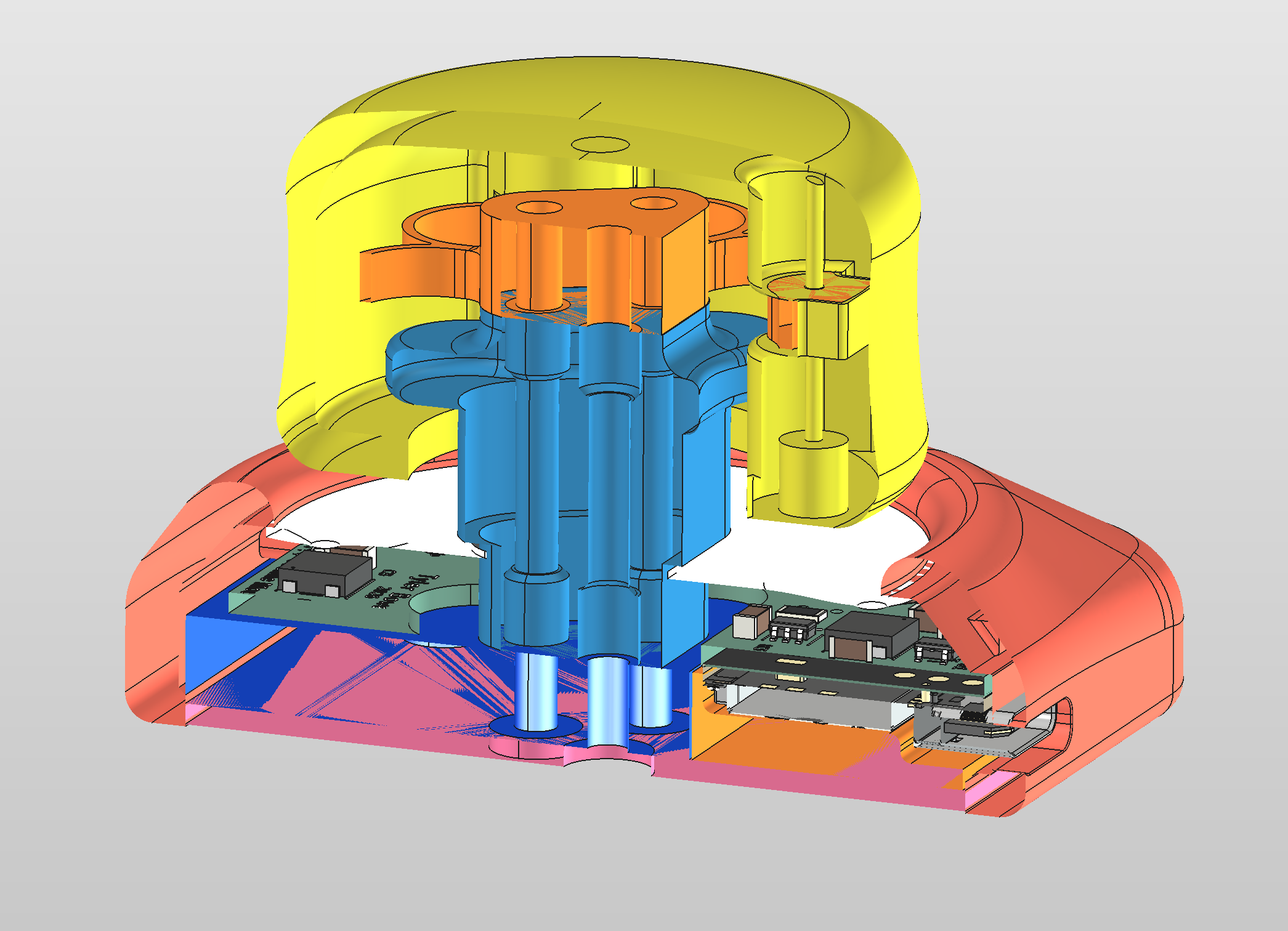
Diffuser: Since the LEDs point directly upwards, they will highlight areas with higher light concentration if used with a flat diffuser. Since light spreads under the inverse square law the diffuser compensates for this by restricting the light intensity near the center and tapering off to the edges. Since these are RGB LEDs, there are actually 3 (sometimes 4) LEDs within the chips so a flat section is used right about the LED module.
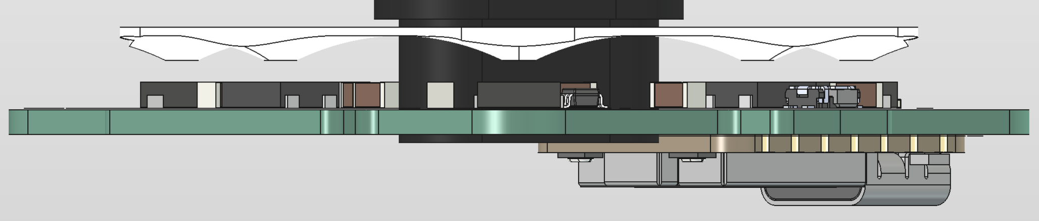
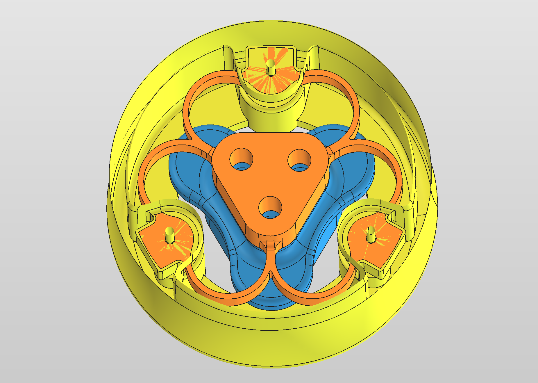
Knob: The knob is a simple rotation of a profile, it has a slight indent to center the user's fingers and cutouts along the bottom edge to meet the base. I debated adding axis ridges, like on the actual space mouse (these help to align the user with mouse movements), and I may do this in the future but haven't yet. The spring is held in with thin rods (paperclips) and the magnets hold the rods in with friction and a small dab of superglue. I used rods instead of screws since the spring is subject to torsion and other forces which would loosen screws with usage.
Spring: The spring is designed to be isotropic, meaning that the same force can be applied across each dimension to achieve the same displacement - e.g. 1N in the +/- X direction should move the same amount when applied in the +/- Y and +/- Z directions. Rotations should behave similarly, though the relationship is moments and angular movement - e.g 1N applied radially should rotate the same number of degrees as the other axis. Isotropicity between translation and rotations is related via \theta \degree = \frac{x}{r} \frac{180}{\pi}. Movements are limited by a kick-out on the knob shaft and hat on the spring which constrain the springs movements, the shaft is designed to be rotated into the shaft with the spring attached, though it is a tight fit.
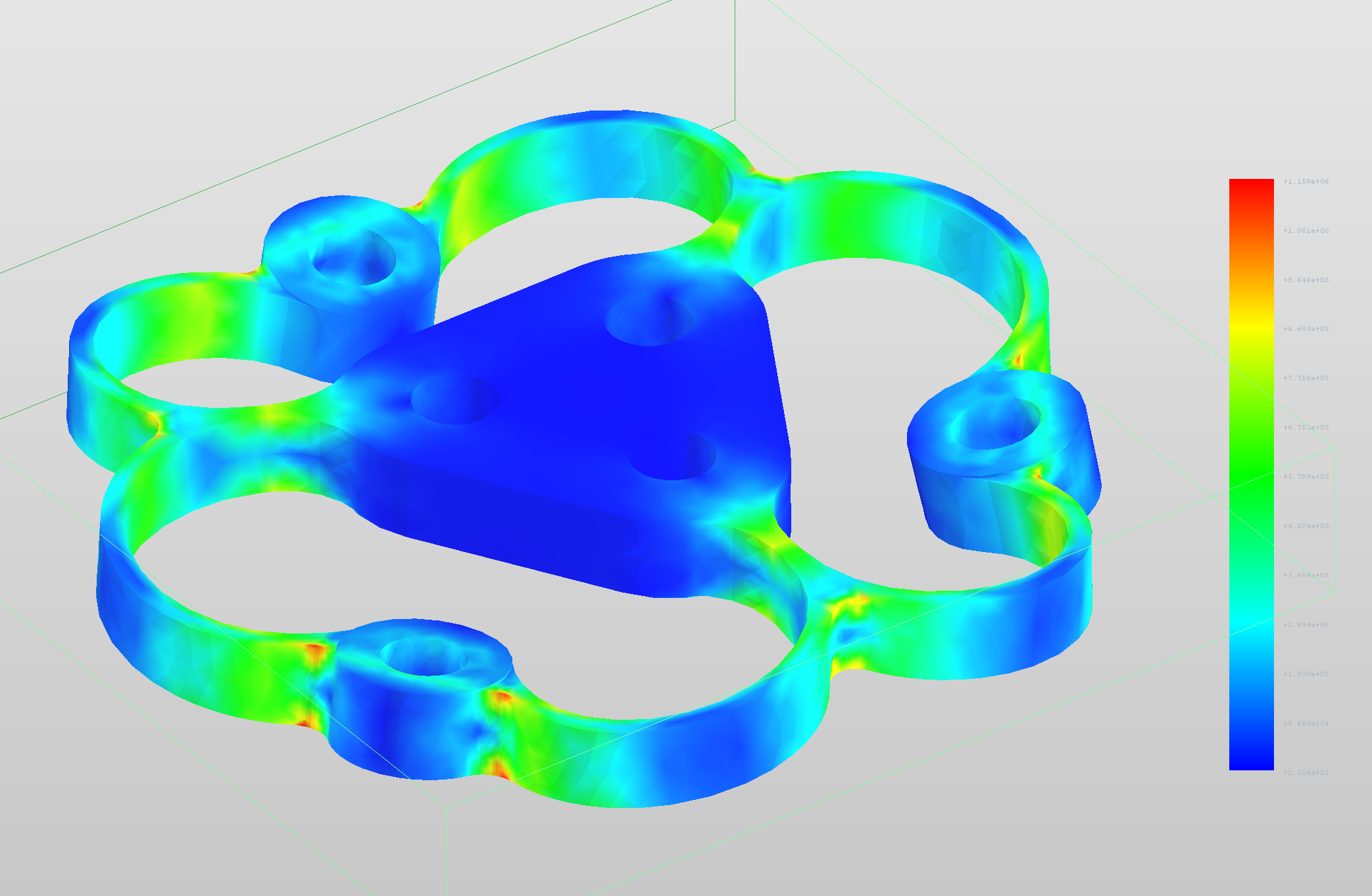
I performed FEA to determine how much stress points on the spring. This does not use any contact constraints between the knob and spring so the results are not completely representative. (I may update this in the future)
Physics Model
There are simple ways to get the knob's movements. It is simple to just take the readings and build a plane from there, but then the movement is non-linear (magnetic force falls at the inverse cube of distance). So to compensate a cubic-linear mapping is used (take the cube root of the measurements) to get a linear scale, then map to a range and at boot apply offsets to center the knob. But there is one more issue with this approach: cross talk (especially during rotations about the Z axis) can drift from their true place. My approach is completely different, I use a physics-based model to iteratively solve for the knob's position by using the magnetic dipole field and the difference between measured and predicted magnetic fields. This model is described below.
1. Forward model:
Magnetic Dipole Field:
- \mu_0 = 4\pi\cdot10^{-7}\ \text{H/m} = permeability of free space
- \vec{r} = position vector from the dipole center to the observer
- r = |\vec{r}| = distance from the dipole center to the observer
- \hat{r} = \vec{r}/r = unit vector from the dipole center to the observer
- \vec{m} = magnetic moment of the dipole
Magnetic Moment (3/16 in dia × 3/16 in height cylinder, N52):
- $B_r = 1.42\ \text{T}$ = residual induction (remanence) of N52
- V = \pi\left(\tfrac{4.7\ \text{mm}}{2}\right)^2 \cdot 4.7\ \text{mm} = 81.54\ \text{mm}^3 = 8.154\times10^{-8}\ \text{m}^3
(4.7mm used instead of 4.7625mm = 3/16in to account for the coating)
We can pull out a fixed term k, using: \vec m = |\vec m|\,\hat m and |\vec m| = B_rV/\mu_0:
k = 1.42T \cdot 81.54mm^3 / 4π = 9.21 T \cdot mm^3 = 9214 mT \cdot mm^3.
Vector \vec r has 3 components, and one sensor gives 3 measurements, so if \hat m (unit vector of moment) is known, the system can be solved.
2. Inverting one dipole:
A dipole has axial symmetry (in this case, about the vector normal to cylindrical face). Because of this, I will use spherical coordinates, r = distance from the origin (sensor), a angle rotating from the z axis c = cos(a) = \hat r \cdot \hat m (normal to the top face of the sensor), and \phi azimuth rotation about the z axis.
Knowns:
Sensor position: \vec{S} = (0, 14.5, 0) mm
Magnet strength: k = 9214 mT \cdot mm^3
Measured field: \vec{B} = (0, 5.091, 20.885) mT
Now to solve for c. Let u be the cosine of the angle between the field and the magnet’s axis.
Quadratic formula:
We know that the magnet is above the sensor, so c > 0. (Durning initialization we can check the sign of the z reading to see if the magnet is flipped up or down; if flipped all readings will be inverted before going into calculations.)
Now to solve for r.
Position:
Example:
Measurements from U3: X -2.26mT, Y -5.12mT, Z 15.40mT
Angle a:
c is negative because the moment points down while \hat r points up. That puts the magnet 13.25\degree off straight up.
Distance r:
Direction \hat r:
Magnet position:
y is flipped due to U3 sensor's location
Summary of Equations
| # | Step | Equation | Purpose |
|---|---|---|---|
| 0 | Constants | k = \dfrac{B_rV}{4\pi} | Magnet strength |
| 1 | Sensor axes → board frame | \vec B_i = \mathbf R_z(\varphi_i)\,(-X_i,\ +Y_i,\ -Z_i) | TMAG5273: +X toward pins 1–3, +Y toward pin 1, +Z into the board |
| 2 | Polarity | \sigma = \operatorname{sign}(B_{z,rest}), then \vec B \leftarrow \sigma\vec B | Makes the moment point up whichever way the magnet is inserted |
| 3 | Remove cross-talk (optional, iterative) | \vec B^{own}_i = \vec B_i - \sum_{j\ne i} k\,\dfrac{3\hat r_{ij}(\hat m\cdot\hat r_{ij}) - \hat m}{r_{ij}^3} | Subtracts the neighbouring magnets' fields |
| 4 | Magnet axis | \hat m = \hat z at rest; \hat m = \mathbf R\hat z when tilted | Direction of the moment |
| 5 | Field magnitude | \lvert\vec B\rvert = \sqrt{B_x^2 + B_y^2 + B_z^2} | Total strength |
| 6 | Field tilt | u = \dfrac{\vec B\cdot\hat m}{\lvert\vec B\rvert} | Cosine of the field's angle from the magnet axis; cancels k/r^3 |
| 7 | Solve for the angle | s = 3c^2 = \dfrac{(2+u^2) + u\sqrt{u^2+8}}{2} | Inverts u = \dfrac{3c^2-1}{\sqrt{3c^2+1}} |
| 8 | Viewing angle | c = \cos a = +\sqrt{s/3} | + because the magnet is in front of the sensor along \hat m |
| 9 | Distance | r = \left(\dfrac{k\sqrt{s+1}}{\lvert\vec B\rvert}\right)^{1/3} | Undoes the 1/r^3 fall-off |
| 10 | Direction (general) | \hat r = \dfrac{\dfrac{r^3}{k}\vec B + \hat m}{3c} | Sensor → magnet unit vector |
| 10′ | Direction (shortcut, \hat m = \hat z only) | \hat r = \sin a\,\dfrac{(B_x,\ B_y,\ 0)}{\sqrt{B_x^2+B_y^2}} + \cos a\,\hat z | Same result while the knob isn't tilted |
| 11 | Magnet position | \vec M_i = \vec S_i + r\,\hat r | Sensor position plus the vector to the magnet |
The next step is to include the other 2 magnets to remove the cross-talk.
3. Removing cross-talk
Each sensor measures the sum of all three magnet fields, not just its own magnet. While the their influence is small (field strength falls as 1/r^3) the effect changes as the knob is moved so a simple offset does not work. Fields add as vectors, so the total at sensor i is:
- \vec S_i = position of sensor i
- \vec M_j = position of magnet j
- \vec r_{ij} = vector from magnet j to sensor i (the dipole formula needs dipole → observer)
The single-dipole inversion (sec 2) only works on one magnet's field. So before inverting, the neighboring fields are subtracted:
The neighbours' positions \vec M_j are needed for this, but they are what we're solving for. Because cross-talk is small (<5%), we can iterate:
- Pass 1: invert each sensor with no correction for first estimate of \vec M_1, \vec M_2, \vec M_3
- Pass 2+: use those estimates to compute and subtract the cross-talk, then invert again
- Repeat until the positions stop changing (several passes)
Each pass shrinks the error by some magnitude. Most error in the estimated neighbor positions enters through the small cross-talk term (EMI from component placement can also cause issues).
Geometry
Sensors are placed at radius 14.5 mm, however the hall effect element placements are not in the center of the package. The true position is slightly offset according to the docs (pg 13):
- 1.85 mm from the pin-1 end, 2.9mm package height = 1.45 mm to center, so 0.40 mm past the package center, toward pin 3 (radially inward)
- 0.68 mm from the pins 1–3 edge, 1.6mm package width = 0.8mm to center, so 0.12 mm from the package center, toward pins 1–3.
- 0.73 mm below the top of the package (side view). This plane is z = 0.
Magnets at rest, at radius 16 mm and height h:
This is a lot to do by hand, so instead it can be done in Python:
Code
import numpy as np

K = 1.42 * np.pi * 2.35**2 * 4.7 / (4 * np.pi) * 1000# B_r V / 4pi  (mT*mm^3)
S = np.array([[-0.12, 14.1, 0], [12.271, -6.946, 0], [-12.151, -7.154, 0]]) # Hall elements (mm)
M_REST = np.array([[0, 16, 0], [13.852, -8.008, 0], [-13.852, -8.008, 0]]) # magnets at rest
PHI = np.radians([0, -120, 120]) # footprint rotation
m = np.array([0, 0, 1.0]) # magnet axis

def to_board(raw, i): # TMAG5273 axes -> board frame
    c, s = np.cos(PHI[i]), np.sin(PHI[i])
    x, y, z = -raw[0], raw[1], -raw[2]
    return np.array([c * x - s * y, s * x + c * y, z])

def dipole(r): # field at r from a magnet
    d = np.linalg.norm(r); u = r / d
    return K * (3 * u * (m @ u) - m) / d**3

def invert(B, Si):# section 2
    Bn = np.linalg.norm(B); u = B @ m / Bn
    s = ((2 + u*u) + u * np.sqrt(u*u + 8)) / 2
    c = np.sqrt(s / 3); r = (K * np.sqrt(s + 1) / Bn) ** (1/3)
    return Si + r * (B * r**3 / K + m) / (3 * c)

B = [to_board(b, i) for i, b in enumerate([[2.26,5.12,-15.40]])]
B = [np.sign(B[0][2]) * b for b in B] # polarity
n = len(B)

M = M_REST.astype(float)
for p in range(1, 6):
    old = M.copy()
    for i in range(n):
        xt = sum(dipole(S[i] - old[j]) for j in range(3) if j != i) if p > 1 else 0
        M[i] = invert(B[i] - xt, S[i])
    M[n:, 2] = M[:n, 2].mean() # unmeasured magnets: rest, same height
    print(f"pass {p}: " + "  ".join(f"M{i+1}={np.round(M[i], 3)}" for i in range(n)))
    if p > 1 and np.abs(M - old).max() < 0.005: break
pass 1: M1=[-1.076 16.267 10.055]
pass 2: M1=[-1.023 16.434  9.86 ]
pass 3: M1=[-1.022 16.43   9.859]
We can see that the final magnet position, after cross-talk is removed, changes the position by ~2%. However, we have a problem because when we solve each position independently, the magnets relative positioning no longer matches up.
4. Levenberg–Marquardt least squares fit
Solving each magnet on its own lets the three positions drift apart. The magnets are fixed into a rigid knob, so their spacing never changes as are the sensors to the PCB. While component positions will vary due to manufacturing differences (I am hand soldering) we can at least parallelize the calculation then use a least squares solver to find the best fit.
Unknowns: (the knob pose)
- x, y, z = position of the knob center.
- \phi, \theta, \psi = roll, pitch, yaw
Magnet positions:
For a given pose, the magnets and their axis in the board frame are:
Residuals:
Stack the differences into one vector of 9 residuals:
The best pose minimizes the sum of squared residuals:
There are 9 equations and 6 unknowns, so the system is over-determined. (2 magnets and 2 sensors could be used) The 3 extra equations average out noise and the leftover residual shows how well the model fits.
\mathbf r(\mathbf p) is non-linear (because of 1/r^3, the unit vectors and the rotations), so it is solved iteratively. Near the current guess, the residual is approximately linear. \mathbf J (the Jacobian) says how each of the 9 readings change when each of the 6 pose values change. It is computed numerically: nudge each pose value by a tiny amount \varepsilon and see how the residuals change. The update step is:
- Small \lambda: Gauss–Newton step, fast compared to large \lambda.
- Large \lambda: this is a short step similar to gradient descent.
Each iteration:
- Compute \mathbf r and \mathbf J at the current \mathbf p
- Solve for \Delta\mathbf p (a 6×6 linear system)
- If F(\mathbf p + \Delta\mathbf p) < F(\mathbf p): accept the step and set \lambda \leftarrow \lambda/10 (trust the linear model more)
- Otherwise: reject the step, set \lambda \leftarrow 10\lambda (take a shorter, safer step) and try again
- Stop when \Delta\mathbf p is negligible
Starting from the rest pose (or, in firmware, the previous frame's pose), it converges in a handful of iterations.
Code
import sys
import numpy as np

K = 1.42 * np.pi * 2.35**2 * 4.7 / (4 * np.pi) * 1000            # B_r V / 4pi  (mT*mm^3)
S = np.array([[-0.12, 14.1, 0], [12.271, -6.946, 0], [-12.151, -7.154, 0]])   # Hall elements (mm)
Q = np.array([[0, 16, 0], [13.852, -8.008, 0], [-13.852, -8.008, 0]])        # magnets in knob frame
PHI = np.radians([0, -120, 120])

def to_board(raw, i):
    c, s = np.cos(PHI[i]), np.sin(PHI[i]); x, y, z = -raw[0], raw[1], -raw[2]
    return np.array([c * x - s * y, s * x + c * y, z])

def rot(rx, ry, rz):
    cx, sx, cy, sy, cz, sz = np.cos(rx), np.sin(rx), np.cos(ry), np.sin(ry), np.cos(rz), np.sin(rz)
    return (np.array([[cz, -sz, 0], [sz, cz, 0], [0, 0, 1]]) @ np.array([[cy, 0, sy], [0, 1, 0], [-sy, 0, cy]])
            @ np.array([[1, 0, 0], [0, cx, -sx], [0, sx, cx]]))

def magnets(p): # p = x, y, z, roll, pitch, yaw [, k scale]
    R = rot(*p[3:6]); return Q @ R.T + p[:3], R @ [0, 0, 1]

def model(p): # all 9 readings: every magnet at every sensor
    M, m = magnets(p); k = K * (p[6] if len(p) > 6 else 1)
    out = []
    for s in S:
        B = 0
        for Mj in M:
            r = s - Mj; d = np.linalg.norm(r); u = r / d
            B = B + k * (3 * u * (m @ u) - m) / d**3
        out.append(B)
    return np.concatenate(out)

def fit(b, p): # Levenberg-Marquardt
    for _ in range(50):
        r = model(p) - b
        J = np.array([(model(p + e) - model(p)) / 1e-6 for e in np.eye(len(p)) * 1e-6]).T
        A = J.T @ J; dp = np.linalg.solve(A + 1e-3 * np.diag(np.diag(A)), -J.T @ r)
        p = p + dp
        if np.abs(dp).max() < 1e-8: break
    return p, np.sqrt(np.mean((model(p) - b) ** 2))

vals = np.array([-0.80, 4.68, -14.88, 0.37, 3.83, -19.97, -0.95, 2.48, -19.11])
B = np.concatenate([to_board(vals[3*i:3*i+3], i) for i in range(3)])
B *= np.sign(B[2])                               # polarity

for name, p0 in [("pose (k fixed)", np.r_[0, 0, 10, 0, 0, 0]), ("pose + strength", np.r_[0, 0, 10, 0, 0, 0, 1])]:
    p, rms = fit(B, p0.astype(float))
    M, _ = magnets(p)
    print(f"\n{name}: rms residual {rms:.3f} mT" + (f", strength x{p[6]:.3f}" if len(p) > 6 else ""))
    print(f"  center ({p[0]:.3f}, {p[1]:.3f}, {p[2]:.3f}) mm   roll {np.degrees(p[3]):.2f}  "
          f"pitch {np.degrees(p[4]):.2f}  yaw {np.degrees(p[5]):.2f} deg")
    for j in range(3):
        print(f"  M{j+1} = ({M[j][0]:.3f}, {M[j][1]:.3f}, {M[j][2]:.3f})   radius {np.hypot(*M[j][:2]):.3f}")
pose (k fixed): rms residual 0.759 mT
  center (0.183, 0.430, 9.684) mm   roll 1.33  pitch 0.48  yaw -0.25 deg
  M1 = (0.257, 16.425, 10.054)   radius 16.427
  M2 = (13.998, -7.638, 9.382)   radius 15.946
  M3 = (-13.705, -7.515, 9.615)   radius 15.630

pose + strength: rms residual 0.428 mT, strength x1.516
  center (0.233, 0.417, 11.117) mm   roll 1.56  pitch 0.55  yaw -0.36 deg
  M1 = (0.337, 16.411, 11.553)   radius 16.415
  M2 = (14.032, -7.673, 10.767)   radius 15.993
  M3 = (-13.670, -7.501, 11.031)   radius 15.593
Results:
| Independent (section 3) | Rigid LM fit | |
|---|---|---|
| \vec M_1 (mm) | (0.22, 16.40, 10.06) | (0.26, 16.43, 10.05) |
| \vec M_2 (mm) | (13.53, −7.54, 9.44) | (14.00, −7.64, 9.38) |
| \vec M_3 (mm) | (−13.21, −7.40, 9.67) | (−13.71, −7.52, 9.62) |
| Spacing (mm) | 26.7–27.4 (drifts) | 27.70–27.72 |
| Knob pose | ... | x 0.18, y 0.43, z 9.68 mm; roll 1.33°, pitch 0.48°, yaw −0.25° |
5. Implementation
- Calibrate at rest (and when user holds both buttons). Run the fit and keep the rest pose \mathbf p_0 and the leftover residual \vec o = \vec B_{rest} - \vec B^{model}(\mathbf p_0) as a fixed offset. To absorb geometry errors like the 0.5 mm above, plus sensor offsets and dipole-model error.
- Every frame: fit \mathbf r(\mathbf p) = \vec B^{model}(\mathbf p) + \vec o - \vec B, starting from the previous frame's pose (2–3 iterations is enough), and report \mathbf p - \mathbf p_0.
Firmware
There isn't much to cover here since most comes from the model section above. The code adds software debounce for the buttons, calibration processes with visual feedback through the LED ring (hold both buttons for 3s to recalibrate), value tuning, and HID interfacing. The code can be found here.